How Fed-Joint combines sensor trends and failure histories across sites, what its simulated-engine results show, and how to evaluate maintenance value.
Figures open at full size. Wide tables scroll sideways.
A plant with a small fleet may have years of sensor readings and very few complete failure histories. Another plant may have the missing examples, but neither organization wants to hand over its operating data. Training separately wastes potentially useful experience; centralizing everything may be impractical.
Fed-Joint addresses that problem by connecting two kinds of evidence: how a machine’s condition changes over time, and when machines actually fail. Sites collaborate by exchanging model parameters while retaining their raw sensor and failure records locally.
The research supports a specific opportunity: improving remaining-life estimates when local histories are limited and degradation is nonlinear. It does not demonstrate reduced downtime in operating factories, and keeping records local does not by itself establish privacy compliance. Those distinctions determine what a team should test next.
A rising temperature or changing vibration signal can suggest deterioration. Maintenance planning needs another step: translating the evolving condition into a probability of failure and an estimate of remaining useful life.
The Fed-Joint method links these steps. First, a multi-output Gaussian process models the degradation signals. In practical terms, this is a flexible way to learn related curves without requiring every machine to follow a predetermined straight line or quadratic shape. Information shared across units can help estimate how a partially observed curve is likely to develop.
Second, a survival model connects the estimated condition to failure risk. Survival analysis can use both failed assets and assets that were still running when observation ended. The latter records are not failures and are not proof of indefinite reliability: they tell the model only that the asset survived to that point. This is called right-censoring.
Together, the components estimate how much useful life remains and the chance of failure within a future window. Those outputs answer different maintenance questions. Average remaining life helps with longer-term scheduling; near-term failure probability may be more relevant to whether an asset can wait until the next service opportunity.
The method is trained in two stages: the degradation model first, followed by the survival model using the estimated degradation patterns. Each stage alternates local updates with central aggregation.
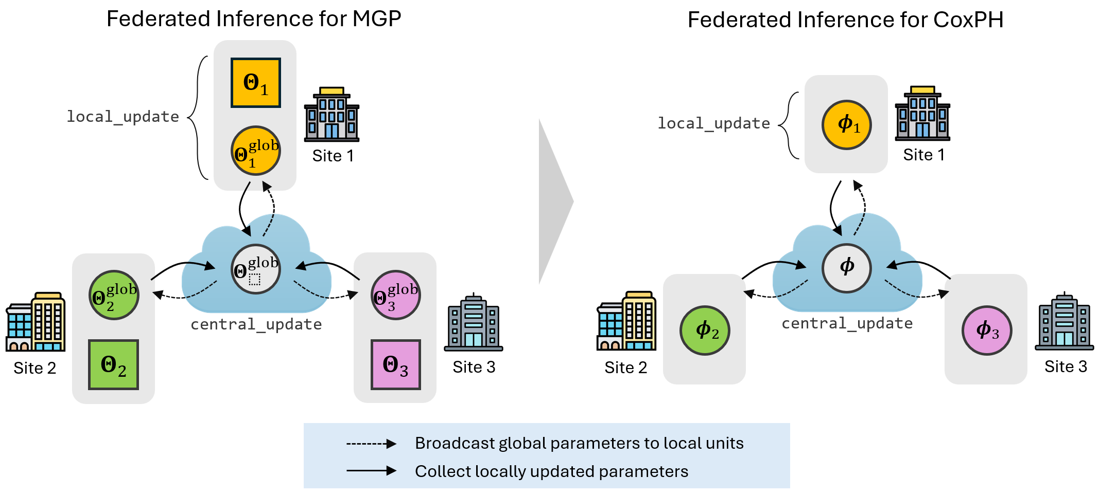
Original Figure 2 from Jeong, Yue and Chung. The left loop learns degradation patterns; the right learns their relationship to failure. Arrows carry updated model parameters and shared parameters, rather than raw machine histories. Source diagram.
Each site fits its portion of the model to its own observations. It sends the parameters designated for sharing to a central coordinator, which combines the updates and sends the shared result back. Some degradation-model parameters remain local, allowing units to retain their own characteristics. The process repeats for the survival component.
The intended benefit is easiest to see early in an asset’s life. A local site may have observed only the relatively flat beginning of a degradation curve. Related histories elsewhere contain the later acceleration. Sharing what the model learns from those histories can improve the forecast before the local asset has accumulated the same evidence.
This still depends on a meaningful relationship between the participating assets. Sharing more data-derived information is not automatically helpful if the sites use incompatible sensors, record different failure definitions or operate under substantially different conditions.
The researchers first construct synthetic degradation patterns, including curves that a simple polynomial model struggles to represent. They compare Fed-Joint with a centralized version, an independent model trained locally, and a local model that assumes a quadratic growth pattern.
The following original panels show the federated and independent versions on one nonlinear example. Gray observations stop around month 30; the later dashed trajectory shows what happened in the simulated signal. The red curve is each model’s estimate.
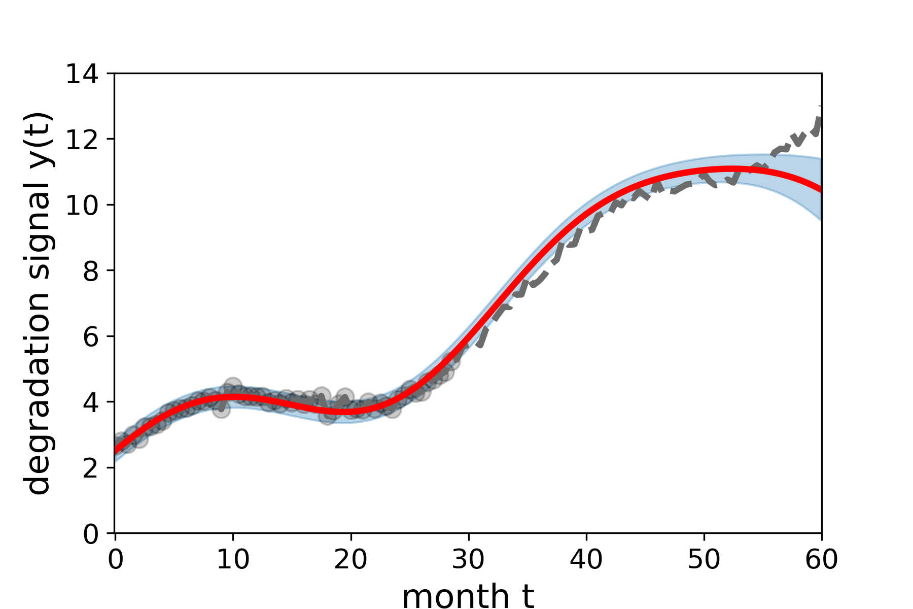
Original Figure 5(a): Fed-Joint. Sharing information helps the forecast follow the later rise in this example, although it still misses the final increase. Source comparison.
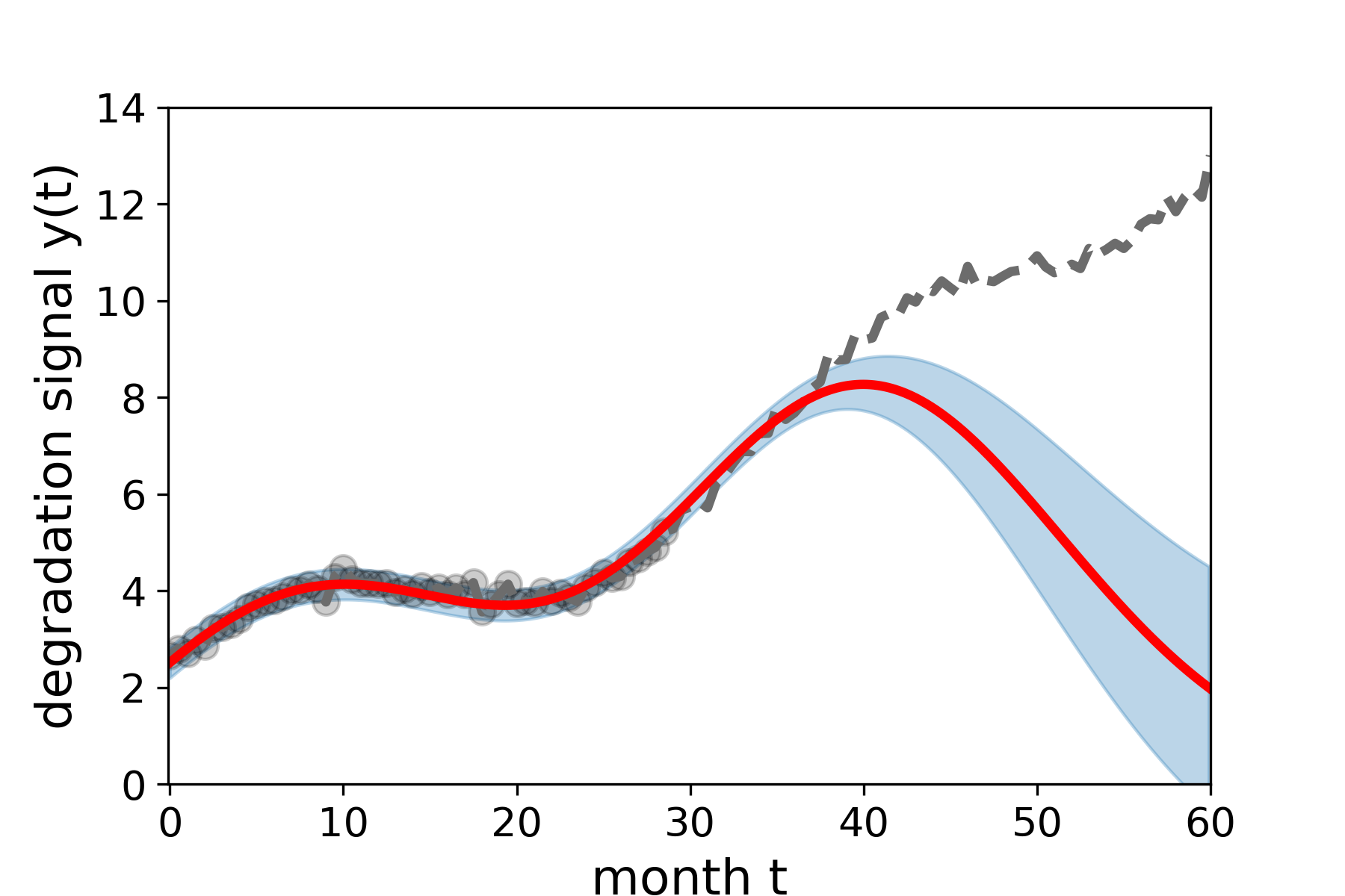
Original Figure 5(c): the independent model. It uses the same general modeling approach without learning from other sites. Its later forecast diverges more sharply. These are illustrative trajectories from the simulation, not measured factory performance.
The comparison explains the method’s purpose better than a generic claim about “more accurate AI.” A flexible model still has to infer the unseen part of a curve. Related histories can supply information that one site lacks. The centralized version also performs strongly, and the quadratic local model can miss the nonlinear shape altogether; the paper does not establish that federation is inherently more accurate than access to all the data.
The second evaluation uses NASA’s C-MAPSS turbofan degradation dataset. Despite the industrial setting, this dataset is generated by simulation. The study uses FD001: a single component’s degradation under constant operating conditions.
From its 100 engine histories, each repeated experiment assigns 20 units to a testing site and 20 each to two training sites. Predictions use 30%, 50% or 70% of the testing units’ histories. The experiment is repeated 20 times, and four informative sensors are evaluated separately.
| Sensor | Method | |||
|---|---|---|---|---|
| 4 | Fed-Joint | 30.71 (4.89) | 24.82 (3.12) | 21.16 (3.84) |
| Cen-Joint | 32.65 (6.62) | 26.35 (4.53) | 20.56 (3.48) | |
| 15 | Fed-Joint | 30.72 (3.56) | 24.58 (3.15) | 20.50 (3.03) |
| Cen-Joint | 32.13 (4.61) | 24.89 (3.07) | 20.08 (2.96) | |
| 17 | Fed-Joint | 32.31 (6.27) | 24.86 (4.32) | 20.81 (2.74) |
| Cen-Joint | 33.54 (7.05) | 26.05 (4.68) | 20.48 (2.67) | |
| 20 | Fed-Joint | 32.09 (4.50) | 24.65 (3.22) | 19.27 (2.52) |
| Cen-Joint | 32.23 (4.30) | 24.73 (3.14) | 19.18 (2.58) |
Original Table 4. Values are mean absolute errors in estimated remaining life, in operating cycles; lower is better. Parentheses contain standard deviations across the 20 experiments. The α columns indicate how much of the history is available. Original table.
For sensor 4, Fed-Joint’s mean error falls from 30.71 cycles with 30% of the history to 21.16 with 70%. The centralized version moves from 32.65 to 20.56. The results are close, and which method is lower changes with how much history is available. That supports federation as a way to approach the centralized result in this setup, rather than a claim that it always beats centralization.
The engine case compares those two methods; it does not independently demonstrate a win against every local maintenance model a company might already use. Nor does it test actual maintenance scheduling, spare-parts inventory or avoided breakdowns. Prediction quality is the beginning of that business case.
The most suitable starting point is a group of sites with comparable equipment and a genuine obstacle to pooling records. Before choosing infrastructure, align sensor meanings, units, timestamps, operating regimes and the definition of failure. A planned replacement and an observed failure should not silently become the same training label.
A practical evaluation should hide the later portion of complete historical records, predict from the earlier portion, and compare with what subsequently happened. Hold out assets rather than scattering observations from the same asset across training and evaluation. Compare local-only learning, federation and—where permitted—a pooled reference. Report results for each site as well as the overall average.
Then translate predictions into the decision that matters. A forecast that is late by ten cycles may be far more costly than one that is early by ten, even though an average absolute-error metric treats them equally. Test warning lead time, missed failures and unnecessary interventions under the actual maintenance policy.
Privacy also remains an engineering requirement. The paper keeps raw records local, but model-parameter sharing is not presented as a formal guarantee against information leakage. Differential privacy is identified as future work. The practical question is what each participant can infer from the exchanged updates, not merely whether raw files move.
Our HVAC control analysis addresses another aspect of learning from changing equipment conditions. It concerns choosing control actions; Fed-Joint concerns forecasting deterioration and failure. A useful forecast and a safe operating decision require separate validation.
Begin with an existing local prognostics model and a reproducible evaluation dataset. If failure labels or sensor alignment are unreliable, adding distributed training will make the system harder to diagnose without resolving the underlying problem.
For a research implementation, Algorithm 1 in the paper specifies the two training stages and the split between local updates and central aggregation. The Gaussian-process component and survival likelihood need to be implemented and checked together; a generic federated-learning example is not a ready-made Fed-Joint implementation.
Flower’s strategy interfaces can support coordinating rounds and aggregation in a custom implementation. Its evaluation aggregation guidance is relevant when combining results from participating sites. These are infrastructure components, not substitutes for the paper’s statistical model or privacy design.
A sensible first run simulates the sites within a controlled environment, verifies that local-only and pooled baselines are reproduced, then introduces the parameter exchange. Only after those results are understood should the team add the operational burden of separate environments, access controls, unreliable connectivity and recovery from interrupted rounds.
Fed-Joint’s value lies in the combination: flexible degradation forecasts, failure-event modeling and collaboration across data boundaries. It gives a team a concrete alternative to choosing between isolated local models and a central data lake.
We would pursue it where sites have compatible assets, limited individual failure histories and a measurable reason to collaborate. We would first demand evidence that the improvement survives realistic differences between sites and changes a maintenance decision. Near-centralized prediction accuracy in a simulation is encouraging; it is not yet an uptime or compliance outcome.
Fed-Joint: Joint Modeling of Nonlinear Degradation Signals and Failure Events for Remaining Useful Life Prediction using Federated Learning, Cheoljoon Jeong, Xubo Yue and Seokhyun Chung. arXiv version 1, submitted 17 March 2025. Original diagrams, trajectory panels and the results table above come from this version.
Compare another federated-learning application: exchanging model information across sketch collections.
Evaluate whether a model reveals membership in its training data, regardless of architecture.
Explore how inspection teams can identify predictions that need a second look.