Compare AI scheduling, dispatching rules and solvers using the same constraints. Research explains feasibility, performance gaps and practical evaluation.
Select a figure to open it at full size.
A production schedule can look efficient and still be impossible to run. A machine may be free before its incoming part is ready. The fastest machine for one operation may need a lengthy changeover. An assembly may depend on two different jobs finishing first.
For manufacturing teams evaluating AI scheduling, the first question is whether competing systems represent those constraints correctly. Only then does a shorter schedule mean anything.
Job Shop Scheduling Benchmark addresses that comparison problem. Reijnen and colleagues provide a shared environment for testing dispatching rules, mathematical solvers, genetic algorithms and deep reinforcement learning. Its results give a useful warning: learning-based scheduling deserves a fair test, but conventional solvers deserve a place in that test too.
A job consists of operations that must run in a permitted order. Machines can process only a limited set of operations, and generally cannot process two at once. A common objective is to minimize makespan: the time from starting the schedule until the last operation finishes.
Real factories add complications. In a flexible job shop, an operation can run on alternative machines, with different processing times. Sequence-dependent setup means changing from one operation to another takes additional time. Assembly constraints mean an operation may wait for predecessors from several jobs. Dynamic arrivals mean the full workload is not known at the beginning.
The researchers build these concepts around reusable job, operation, machine and environment objects. Their environment and configuration examples allow methods to receive the same instance instead of relying on separate, subtly different problem definitions. A simulation environment also supports dynamic job arrivals.
That is the important contribution: a common place to expose differences between methods. Support in the environment does not mean every included scheduling algorithm handles every constraint. The paper’s method matrix shows gaps, especially for more complicated variants.
The paper’s custom configuration in Listing 4 describes three jobs, two machines and six operations. Operation 0 takes 10 time units on the first machine or 20 on the second. Its successor, operation 1, takes 25 or 19 respectively.
Choosing the quickest machine for each operation would send the first operation to machine 1 and the second to machine 2. But operation 1 cannot begin before operation 0 finishes, and machine 2 may already be occupied. Another job has an operation that takes 37 units on machine 1 but only 21 on machine 2. Both jobs therefore compete for the same attractive capacity.
The configuration also contains setup-time matrices. These describe the time required to switch between particular operations on each machine. Processing speed alone cannot tell us which assignment produces the earliest overall finish. We must consider availability, dependencies and the sequence already assigned to each machine.
The paper’s assembly example makes the dependency problem visible:
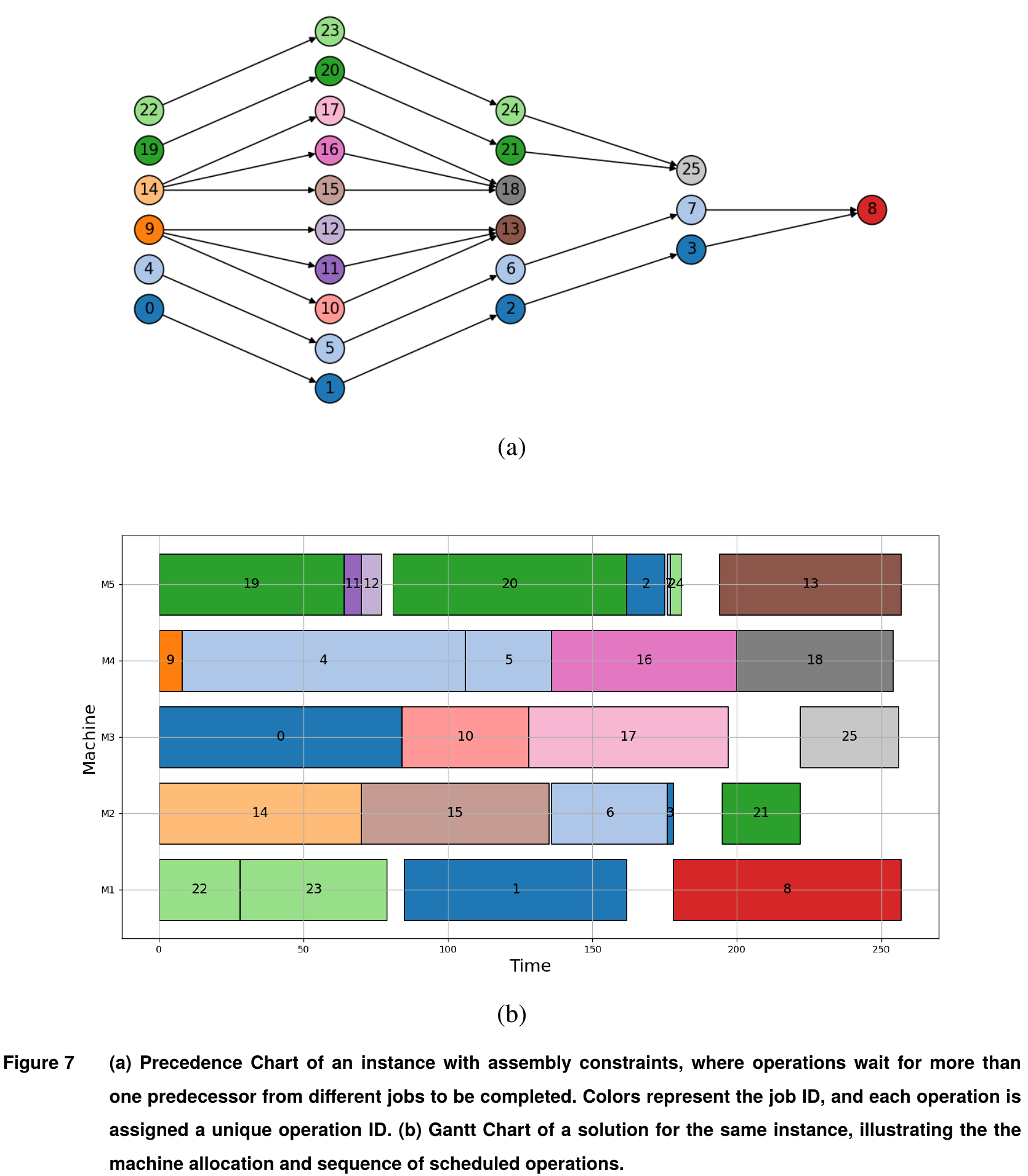
Operation 8 depends on operations 3 and 7; operation 25 depends on 21 and 24. The bars below show when each operation occupies a machine. Empty space can be the consequence of waiting for required work, rather than a scheduler simply overlooking idle capacity. For an operator, that distinction separates an explainable schedule from an attractive but infeasible one.
The researchers compare methods on job-shop, flow-shop and flexible job-shop instances. Their summary reports the gap between each method’s makespan and the best-known solution. A smaller gap is better; it is not a percentage increase in factory output.
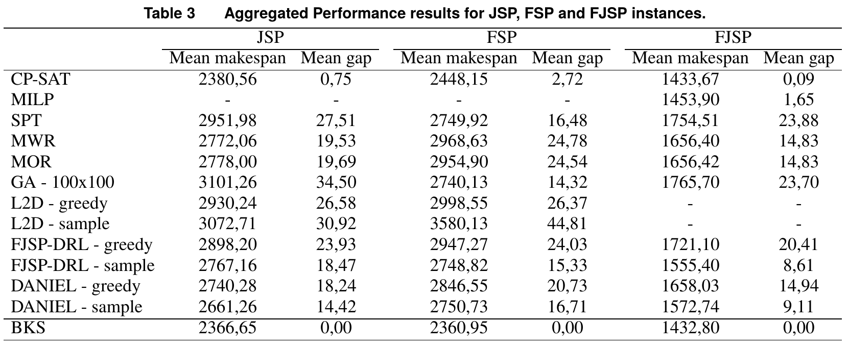
CP-SAT’s mean gaps are 0.75% for job shops, 2.72% for flow shops and 0.09% for flexible job shops. The sampled DANIEL learning method records 14.42%, 16.71% and 9.11%. On flexible job shops, sampled FJSP-DRL improves on the simple most-work-remaining rule: an 8.61% gap versus 14.83%.
These are reasons to benchmark several approaches, not a universal ranking for deployment. The solver receives up to an hour per instance. A dispatching rule makes a much cheaper local choice, while a trained policy moves some computational work into training. A factory needing a response in seconds faces a different decision from one preparing tomorrow’s schedule overnight.
The historical experiment also uses particular instance families and trained models. Your machine eligibility, setups, disruptions and objective may change the comparison. Minimizing the last completion time is not automatically the same as minimizing late customer orders.
The authors’ open scheduling environment is the natural starting point for reproducing this comparison. Use its instance parsers and configurations to express a small representative workload, then run a dispatching-rule baseline before adding a solver or learned policy.
Google OR-Tools’ job-shop example provides a separate starting point for precedence and machine non-overlap constraints. It is useful if you want to build directly around CP-SAT; it does not remove the work of modeling your additional factory constraints.
For a practical evaluation, freeze a set of historical workloads and give each candidate the same decision deadline. Check schedule feasibility independently, then compare completion time, overdue jobs, computation time and recovery after a machine becomes unavailable. Keep training cost and inference time separate. A method that slightly improves makespan but repeatedly misses the replanning deadline may be the weaker operating choice.
Start in shadow mode: generate schedules alongside the existing process and have planners identify missing constraints. Fix the model of the factory before interpreting small performance differences. Our research on adaptive resource allocation examines a related issue: decisions must account for the conditions under which resources are actually available.
The best reason to use this research is to improve the selection process. It gives teams a way to compare AI with established optimization and simple rules without treating “AI” as the outcome they must justify.
Choose a learned scheduler when it meets the real decision deadline and improves the outcomes you care about on representative workloads. Keep a conventional solver when it does the job better. In either case, an explicit, testable model of operational constraints is the asset that survives the next algorithm change.
Job Shop Scheduling Benchmark: Environments and Instances for Learning and Non-learning Methods, Reijnen and colleagues. Version 2, March 17, 2025. This article uses that version’s experiments and original Figure 7 and Table 3.
Optimize drone routes with battery reserves, charging and the full mission in view.
See why generated motion-control code needs behavioral checks beyond valid syntax.