Assess an LSTM job-openings forecast through its original results, data-timing risks and a practical backtest against equal-information baselines.
Figures open at full size. Wide tables scroll sideways.
A model that follows historical job openings closely is useful only if it could have made those predictions with information available at the time. Economic datasets make that condition surprisingly difficult: releases arrive on different schedules, values are revised, and filling a missing entry can accidentally reveal the future.
Kyungsu Kim's study compares a deep learning model with statistical methods for forecasting US Job Openings and Labor Turnover Survey data. Its results make a case for testing multiple economic signals together. They do not yet establish that a deep neural network is the best operational forecasting system—or that an aggregate US forecast can determine your company's hiring needs.
For analytics teams, the practical question is how to test the promising part without inheriting uncertainty in the experiment.
The study asks whether a Long Short-Term Memory network, or LSTM, can predict job openings more accurately by learning relationships among economic indicators over time. Unlike a forecast built only from past openings, the proposed model receives a collection of signals describing the wider economy.
The inputs include measures of prices, consumption, payrolls, industrial output and optimism. These might contain information about future hiring demand that the job-openings series alone does not capture. The research proposition is plausible: when economic conditions change together, a model able to combine their recent histories may track labor demand better. It still needs a comparison that separates the value of those additional inputs from the value of the particular model.
The paper uses monthly data from January 2001 through December 2020, assigning the first 70% to training and the later 30% to testing. That is a historical evaluation, not a forecast of today's labor market. The dataset and processing steps are described in Section 3.
First, missing values are filled using the next available observation—a procedure called backward filling. A CatBoost tree model then ranks features, and the 20 highest-ranked inputs are selected. The selected values are scaled using the median and interquartile range so that very large observations have less influence on scaling than they would under a mean-and-standard-deviation approach.
Those inputs enter a stack of six LSTM layers, described as having 256, 64, 32, 32, 16 and one unit. An LSTM carries an internal state through a sequence, learning what information to retain as it processes successive inputs. Here, the intended output is a numerical estimate of job openings.
The author reports training for 50 epochs and evaluating results across 50 iterations. The paper gives different descriptions of sequence timing—a lag of three in one passage and a time step of two in another—while the results table varies lag settings from one to four. The exact arrangement would need clarification before a faithful reproduction. The architectural idea is understandable; the publication is not a complete implementation recipe. Section 3.2 provides the model description.
The figures below show the same historical target alongside two forecasts. In the Holt–Winters example, the forecast extends an upward trajectory and increasingly overshoots the observed series. The LSTM example follows more of the variation, including a sharp decline near 2020, although it overshoots that decline too.
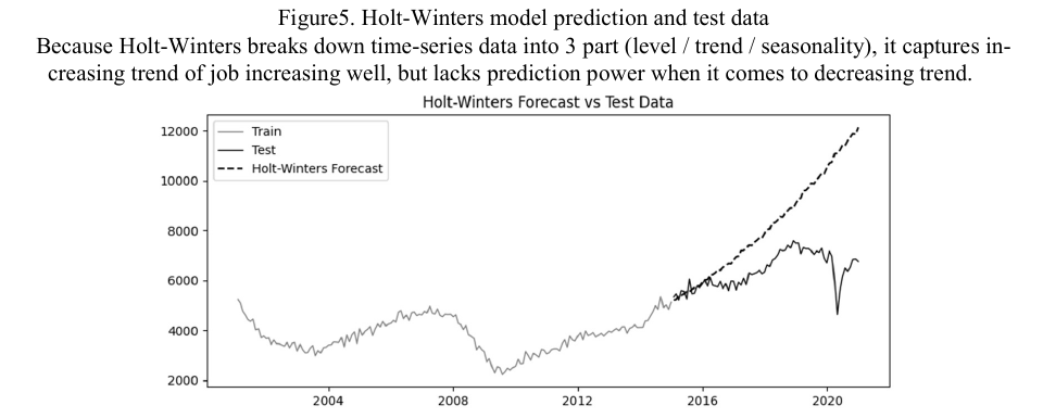
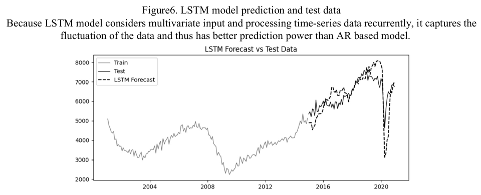
These plots support a limited conclusion: the displayed neural-network forecast tracks this test series more closely than the displayed extrapolation. They do not show whether all inputs were available before each prediction, whether the statistical model was updated through the test period, or whether both methods faced the same forecasting horizon and information constraints.
A sequence that closely follows a historical shock could reflect useful predictive signals. It could also benefit from inputs recorded or revised after the prediction date. The charts alone cannot distinguish those explanations.
The original table reports root mean squared error, which penalizes larger numerical misses more heavily, alongside a percentage-error measure. Lower errors are better, provided the evaluation conditions match.
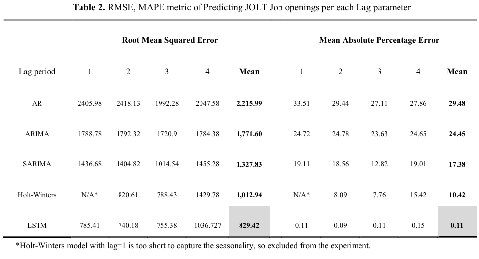
At lag three, LSTM has an RMSE of 755.38 versus 788.43 for Holt–Winters: approximately 4.2% lower. That is a useful improvement to investigate, but much narrower than a claim that deep learning radically transforms forecasting. The table reports larger differences at some other settings, which makes the exact forecasting setup important.
The percentage-error column deserves caution. LSTM's mean is printed as 0.11, while Holt–Winters is 10.42. The paper does not resolve whether these use the same percentage convention. Reading 0.11 as a directly comparable 0.11% would risk manufacturing a dramatic improvement from an unclear reporting scale. We therefore use the matched RMSE comparison rather than that headline.
The appendix provides a lengthy input-data listing, but a usable reproduction also needs the precise target series, release vintages and prediction cutoffs. Those details determine whether a historical comparison resembles the forecast a team could actually issue. The source data description and listing follow the results table.
Backward filling illustrates the risk. Suppose a monthly indicator is missing at a forecast cutoff and the next observation arrives a month later. Filling the earlier gap with that later value gives the historical model information the deployed system would not have possessed. This is a possible failure of the stated method; the paper does not provide enough timing detail to establish exactly where it occurred.
Feature selection and scaling have a similar boundary. Rankings, medians and other learned preprocessing values must come from the training period. Otherwise the supposedly unseen future influences the pipeline before the model predicts it. The paper does not clearly document that boundary for every step.
The comparison also needs an equal-information baseline. Statistical forecasting does not inherently forbid external economic variables. If the neural model receives those signals while a comparator extrapolates only past openings, a win cannot be assigned solely to the neural architecture.
These are actionable questions for reproduction: freeze what was known at each cutoff, fit the entire pipeline on past data, and compare methods receiving the same eligible inputs. The same distinction between when an event occurred and when information became available also matters in EHR prediction pipelines.
Start with data vintages. The FRED API's real-time-period controls let a team request information as it was known during a specified period, rather than automatically relying on the latest revised series. Use the relevant release history for each input and record the actual forecast cutoff. Vintage access is a component of the test, not a replacement for aligning publication dates across sources.
For a stronger statistical comparator, statsmodels SARIMAX accepts external regressors as well as time-series structure. Compare it with a simple last-observation or seasonal baseline and the proposed LSTM. Only supply future regressor values if they would really be known at prediction time; otherwise forecast them or use appropriately lagged inputs.
Run a sequence of historical forecasting rounds. At each round, train and select features using the past, issue the forecast, save it, and advance the cutoff. Keep the horizon identical across models. Report errors separately during ordinary periods and large disruptions, along with the uncertainty around the forecast. A model that wins only in one unusual period may be a poor general planning tool.
For a staffing or recruiting business, the initial application would be a macroeconomic scenario signal. A national openings forecast could inform a discussion about market conditions. Translating it into company headcount requires a separate model of customer demand, productivity, geography and hiring constraints. The study does not test that translation.
The paper offers a worthwhile hypothesis to reproduce: economic inputs considered together may improve a labor-market forecast. Its reported advantage is not strong enough to skip the reproduction work, particularly with unresolved timing and metric questions.
We would first spend effort on a faithful historical data pipeline and matched baselines. If the LSTM retains an advantage across rolling periods, release vintages and useful forecast horizons, its additional complexity has a stronger justification. If the advantage disappears, the improved backtest has still delivered something valuable: a more honest view of what the organization can predict.
Forecasting Labor Demand: Predicting JOLT Job Openings using Deep Learning Model, by Kyungsu Kim. This article uses arXiv version 1, posted 24 March 2025. Original plots and the results table are reproduced under CC BY 4.0 for analysis; the proposed operational backtest is TechClarity's recommendation.
Check whether prediction inputs were actually available at the moment a decision was made.
Examine a financial model that combines relationships across stocks with changes over time.