Learn how reinforcement learning routes deliveries under capacity constraints, what benchmark gains mean, and what is needed to establish emissions savings.
Select a figure to open it at full size.
A logistics team can reduce planned distance without knowing how much fuel or electricity it will save. Vehicle load, congestion, speed and the road network all affect the relationship. That makes the first decision about AI routing surprisingly important: what exactly should the system optimize?
Mohammadreza Nazari and colleagues demonstrate a reinforcement-learning approach to vehicle routing that learns to serve customers while respecting vehicle capacity. The research offers a concrete mechanism for producing routes quickly. Its reward is shorter travel distance, not measured emissions. Understanding that boundary is essential before turning a routing benchmark into a sustainability claim.
This revision replaces the earlier article’s broad sustainability claims with a routing experiment whose inputs, decisions and comparisons are visible.
Each customer begins with a location and a demand. Each vehicle has a limited load. Visiting a customer changes what remains to be delivered and how much capacity is available; returning to the depot replenishes that capacity.
The model separates those inputs. Locations are static throughout the route. Demand and remaining load are dynamic. An attention-based decoder considers both when choosing the next destination, then updates the state after the choice. Training rewards sequences with lower total Euclidean distance.
Before a destination can be selected, the system masks invalid moves. A customer whose demand is already satisfied should not be visited again. In the standard formulation, a customer whose demand exceeds the remaining load is also unavailable. The policy must return to the depot or choose another feasible customer.

The contribution is more than using a neural network to output a list. The state update and feasibility mask let the same decision rule be applied repeatedly as a route unfolds. The model does not have to relearn the problem after every delivery.
The paper also examines split deliveries. Suppose a vehicle has two units left and a customer needs eight. Under the standard rule, it cannot serve that customer on the current trip. If partial delivery is allowed, it can deliver two now and leave six for a later visit.
The authors enable this behavior by relaxing the relevant mask, rather than retraining the routing model. That is an instructive example of separating a learned preference from a business constraint: the model’s scoring machinery stays the same while the permissible actions change.
But the comparison must change with it. A route that permits split deliveries solves a different problem from one that requires a single visit per customer. A shorter split-delivery route is not evidence that the AI has beaten the mathematical optimum of the original problem. In practice, extra visits may also create service costs or customer inconvenience that distance alone ignores.
The experiments generate customers in a unit square, with integer demands from one to nine. Vehicle capacity varies by problem size. The authors evaluate 1,000 test instances at each size and compare learned routes with established heuristics and an OR-Tools baseline.
The policy can decode greedily or use beam search to retain several promising partial solutions. A beam width of ten improves the search over a single sequence of choices. That extra effort is part of the method and should be included in any runtime comparison.
In the appendix’s results, the 50-customer beam-search version has average route length 11.15, compared with 11.31 for OR-Tools. At 100 customers, the values are 16.96 and 17.16. Those are distances in the synthetic coordinate system, not kilometres traveled by a real fleet.
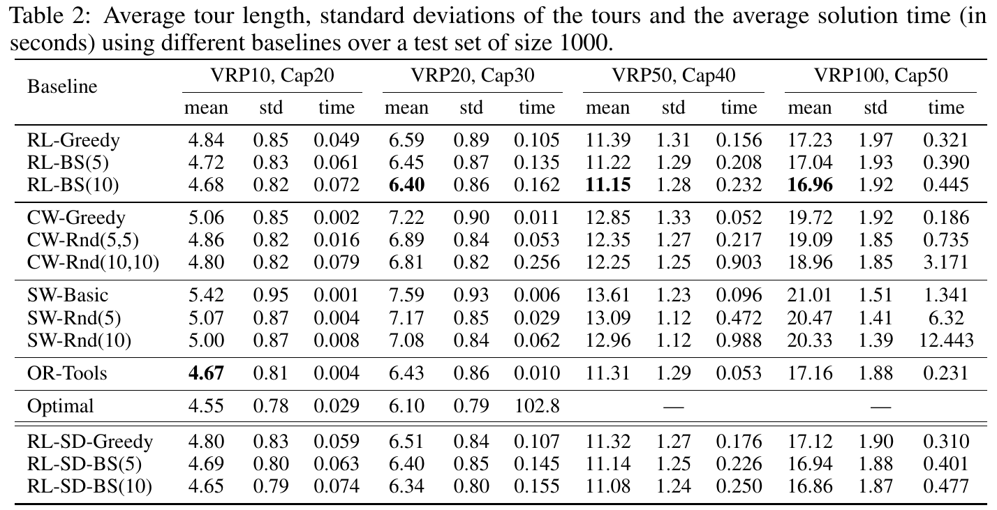
Another result can easily be misread. The learned method beats the OR-Tools route in 60.2% of 50-customer instances and 62.2% of 100-customer instances. That is the share of cases in which it finds the shorter route. It does not mean routes become 60% shorter, or that emissions fall by that amount.
These historical experiments support the proposition that a trained policy can be competitive on a familiar distribution of routing problems. They do not establish superiority over every solver, a current software release or an unfamiliar road network.
The broader green vehicle-routing literature explains why distance is only one input to environmental performance. Load and speed affect energy use; congestion and terrain can change the cost of traveling the same distance. A route’s environmental value therefore depends on the vehicles and operating conditions.
For an electric fleet, the relevant objective might combine energy use, charging availability and on-time delivery. For a diesel fleet, fuel estimates and service constraints may be more useful than a generic distance reward. Those objectives require data and validation; labeling a distance-minimizing model “green AI” does not supply them.
A practical pilot should begin with historical orders and actual vehicle constraints. Run the current planner and the candidate on the same days. Compare distance, estimated or measured energy, late deliveries, capacity violations and computation time. Where possible, calibrate the energy model against telemetry before using it to make environmental claims.
Keep unusual days in the evaluation: dispersed customers, unusually heavy loads, a vehicle outage or demand outside the training range. They test whether the policy has learned useful routing behavior or mainly adapted to a narrow pattern of synthetic demand. Battery-aware drone routing illustrates the same need to make resource constraints explicit.
The authors’ VRP-RL repository is a starting point for reproducing the historical learning approach. It is research code, so dependencies and assumptions need checking before integration. OR-Tools’ capacity-constrained routing examples provide a conventional baseline and a concrete representation of customer demand and vehicle capacity.
Use one shared evaluator for both methods. It should calculate the objective, reject invalid routes and report unserved demand. First reproduce a small instance whose feasibility can be checked by hand. Then add the operation’s time windows, service times and environmental objective. Accept a candidate only if its advantage survives those constraints without shifting costs into missed deliveries or extra visits. This article does not report an executed implementation.
The useful opportunity is a reusable routing policy that can generate competitive plans quickly. The sustainability opportunity comes later, when the optimization objective reflects the fleet’s actual resource use.
Teams should require both pieces of evidence: better feasible routes under a fair comparison, and a defensible connection between those routes and energy or emissions. Without the second, the result is an operational routing improvement, not a demonstrated carbon reduction.
Mohammadreza Nazari, Afshin Oroojlooy, Martin Takáč and Lawrence V. Snyder, Reinforcement Learning for Solving the Vehicle Routing Problem, arXiv version 2, May 21, 2018.
Saba Sabet and Bilal Farooq, Green Vehicle Routing Problem: State of the Art and Future Directions, arXiv version 1, February 3, 2022. Used for the distinction between route distance and environmental objectives.
Optimize drone routes with battery reserves, charging and the full mission in view.
Measure the workload and energy used before making an AI sustainability claim.
Compare learned schedules, rules and solvers under the same operational constraints.